
8.1. Characteristic Function Concept#
The Big Question: What IS a characteristic function, and why does it work?
A characteristic function (CF) is defined as: $\(\phi_X(\omega) = \mathbb{E}[e^{i\omega X}]\)$
This looks mysterious! Let’s build intuition step by step.
Attribution
This educational notebook was developed with assistance from GitHub Copilot (Claude Sonnet 4.5), December 2024. The pedagogical approach, visualizations, and step-by-step explanations were collaboratively created to make characteristic function theory accessible to researchers in chromatography and related fields.
8.1.1. Why Complex Exponentials?#
Euler’s Formula#
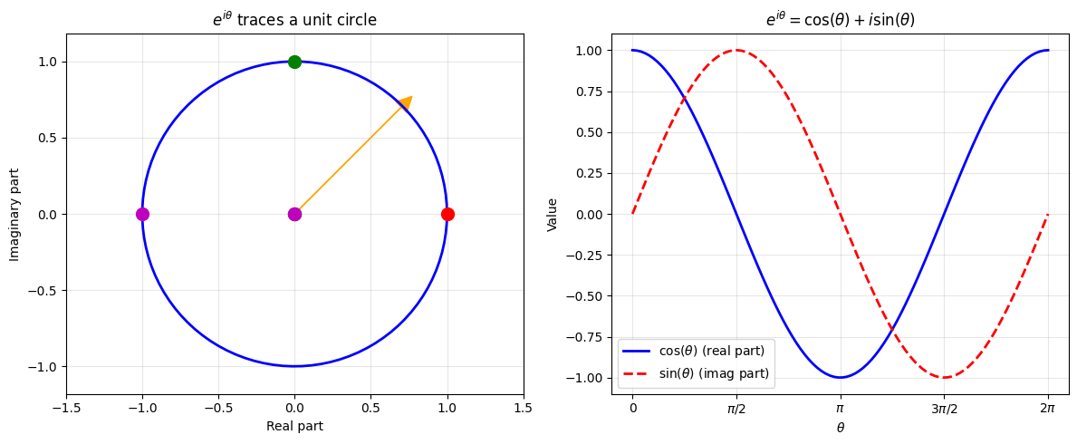
The key is Euler’s formula: $\(e^{i\theta} = \cos(\theta) + i\sin(\theta)\)$
This is a unit vector rotating on the complex plane:
When \(\theta = 0\): \(e^{i \cdot 0} = 1\) (pointing right)
When \(\theta = \pi/2\): \(e^{i\pi/2} = i\) (pointing up)
When \(\theta = \pi\): \(e^{i\pi} = -1\) (pointing left)
When \(\theta = 2\pi\): \(e^{i2\pi} = 1\) (back to start)
So \(e^{i\omega X}\) is a rotating vector where the angle is \(\omega X\).
import numpy as np
import matplotlib.pyplot as plt

# Visualize Euler's formula
theta = np.linspace(0, 2*np.pi, 100)
z = np.exp(1j * theta)

fig, (ax1, ax2) = plt.subplots(1, 2, figsize=(12, 5))

# Complex plane circle
ax1.plot(z.real, z.imag, 'b-', linewidth=2)
ax1.plot([0, 1], [0, 0], 'ro', markersize=10)  # θ=0
ax1.plot([0, 0], [0, 1], 'go', markersize=10)  # θ=π/2
ax1.plot([0, -1], [0, 0], 'mo', markersize=10)  # θ=π
ax1.arrow(0, 0, 0.7, 0.7, head_width=0.1, head_length=0.1, fc='orange', ec='orange')
ax1.set_xlabel('Real part')
ax1.set_ylabel('Imaginary part')
ax1.set_title(r'$e^{i\theta}$ traces a unit circle')
ax1.grid(True, alpha=0.3)
ax1.axis('equal')
ax1.set_xlim(-1.5, 1.5)
ax1.set_ylim(-1.5, 1.5)

# Real and imaginary components
ax2.plot(theta, np.cos(theta), 'b-', linewidth=2, label=r'$\cos(\theta)$ (real part)')
ax2.plot(theta, np.sin(theta), 'r--', linewidth=2, label=r'$\sin(\theta)$ (imag part)')
ax2.set_xlabel(r'$\theta$')
ax2.set_ylabel('Value')
ax2.set_title(r'$e^{i\theta} = \cos(\theta) + i\sin(\theta)$')
ax2.legend()
ax2.grid(True, alpha=0.3)
ax2.set_xticks([0, np.pi/2, np.pi, 3*np.pi/2, 2*np.pi])
ax2.set_xticklabels(['0', r'$\pi/2$', r'$\pi$', r'$3\pi/2$', r'$2\pi$'])

plt.tight_layout()
plt.show()

print("e^(iθ) is a ROTATION by angle θ on the complex plane")
Ignoring fixed y limits to fulfill fixed data aspect with adjustable data limits.
Ignoring fixed y limits to fulfill fixed data aspect with adjustable data limits.
e^(iθ) is a ROTATION by angle θ on the complex plane
8.1.2. What Does the Expectation Mean?#
For a random variable \(X\) with probability density \(f(x)\): $\(\phi_X(\omega) = \mathbb{E}[e^{i\omega X}] = \int_{-\infty}^\infty e^{i\omega x} f(x) dx\)$
Intuition:
Each value \(x\) contributes a rotating vector \(e^{i\omega x}\)
Weighted by probability \(f(x)\)
The CF is the weighted average direction of all these vectors
Key insight: Different distributions create different rotation patterns!
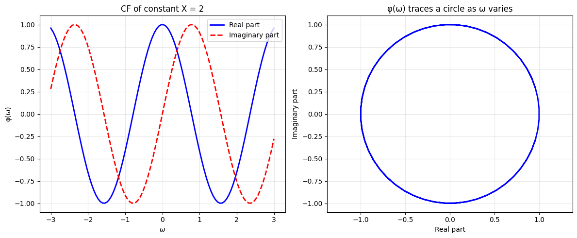
8.1.3. Simple Example 1: Constant Random Variable#
If \(X = c\) (always the same value): $\(\phi_X(\omega) = \mathbb{E}[e^{i\omega c}] = e^{i\omega c}\)$
This is just pure rotation - no averaging needed because there’s no randomness!
# Example: X = 2 (constant)
c = 2
omega_range = np.linspace(-3, 3, 100)
phi = np.exp(1j * omega_range * c)

fig, (ax1, ax2) = plt.subplots(1, 2, figsize=(12, 5))

# Real and imaginary parts
ax1.plot(omega_range, phi.real, 'b-', linewidth=2, label='Real part')
ax1.plot(omega_range, phi.imag, 'r--', linewidth=2, label='Imaginary part')
ax1.set_xlabel(r'$\omega$')
ax1.set_ylabel('φ(ω)')
ax1.set_title(f'CF of constant X = {c}')
ax1.legend()
ax1.grid(True, alpha=0.3)

# Complex plane
ax2.plot(phi.real, phi.imag, 'b-', linewidth=2)
ax2.set_xlabel('Real part')
ax2.set_ylabel('Imaginary part')
ax2.set_title(f'φ(ω) traces a circle as ω varies')
ax2.grid(True, alpha=0.3)
ax2.axis('equal')

plt.tight_layout()
plt.show()

print(f"For constant X = {c}:")
print(f"  φ(ω) = e^(i·{c}·ω) = cos({c}ω) + i·sin({c}ω)")
For constant X = 2:
  φ(ω) = e^(i·2·ω) = cos(2ω) + i·sin(2ω)
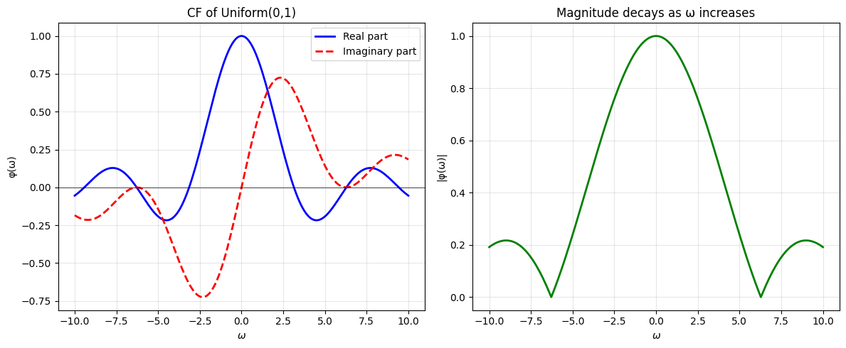
8.1.4. Simple Example 2: Uniform Distribution#
For \(X \sim \text{Uniform}(0, 1)\): $\(\phi_X(\omega) = \int_0^1 e^{i\omega x} dx = \frac{e^{i\omega} - 1}{i\omega}\)$
Intuition:
Values from 0 to 1 contribute vectors at different angles
When averaged, they partially cancel (unlike the constant case)
This creates a decaying pattern as \(\omega\) increases
# Uniform(0,1) characteristic function
def uniform_cf(omega):
    """CF of Uniform(0,1): (e^(iω) - 1)/(iω)"""
    # Handle ω=0 case separately (limit is 1)
    result = np.zeros_like(omega, dtype=complex)
    nonzero = omega != 0
    result[nonzero] = (np.exp(1j * omega[nonzero]) - 1) / (1j * omega[nonzero])
    result[~nonzero] = 1.0
    return result

omega_range = np.linspace(-10, 10, 200)
phi_uniform = uniform_cf(omega_range)

fig, (ax1, ax2) = plt.subplots(1, 2, figsize=(12, 5))

# Real and imaginary parts
ax1.plot(omega_range, phi_uniform.real, 'b-', linewidth=2, label='Real part')
ax1.plot(omega_range, phi_uniform.imag, 'r--', linewidth=2, label='Imaginary part')
ax1.axhline(0, color='k', linewidth=0.5)
ax1.set_xlabel(r'$\omega$')
ax1.set_ylabel('φ(ω)')
ax1.set_title('CF of Uniform(0,1)')
ax1.legend()
ax1.grid(True, alpha=0.3)

# Magnitude (shows decay)
ax2.plot(omega_range, np.abs(phi_uniform), 'g-', linewidth=2)
ax2.set_xlabel(r'$\omega$')
ax2.set_ylabel('|φ(ω)|')
ax2.set_title('Magnitude decays as ω increases')
ax2.grid(True, alpha=0.3)

plt.tight_layout()
plt.show()

print("Notice: The CF 'spreads out' the rotation - vectors at different angles average out!")
Notice: The CF 'spreads out' the rotation - vectors at different angles average out!
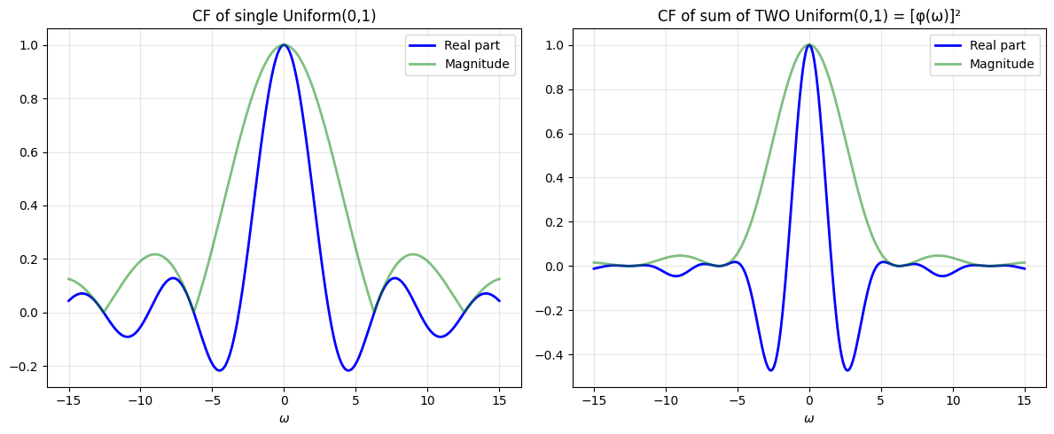
8.1.5. The Magic Property: Sums Become Products!#
This is the KEY reason CFs are useful:
If \(X\) and \(Y\) are independent, then: $\(\phi_{X+Y}(\omega) = \phi_X(\omega) \cdot \phi_Y(\omega)\)$
Why does this work?
Using independence (critical!): $\(= \mathbb{E}[e^{i\omega X}] \cdot \mathbb{E}[e^{i\omega Y}] = \phi_X(\omega) \cdot \phi_Y(\omega)\)$
Intuition:
Adding random variables = convolving their distributions (hard!)
Multiplying CFs = simple multiplication (easy!)
This is why Fourier transform theory is so powerful
# Demonstrate: CF of sum = product of CFs
# Example: Sum of two independent Uniform(0,1) random variables

omega_range = np.linspace(-15, 15, 300)

# CF of single Uniform(0,1)
phi_1 = uniform_cf(omega_range)

# CF of sum of TWO independent Uniform(0,1) = product of CFs
phi_sum = phi_1 * phi_1  # This is φ₁(ω)²

fig, (ax1, ax2) = plt.subplots(1, 2, figsize=(12, 5))

# Single uniform
ax1.plot(omega_range, phi_1.real, 'b-', linewidth=2, label='Real part')
ax1.plot(omega_range, np.abs(phi_1), 'g-', linewidth=2, alpha=0.5, label='Magnitude')
ax1.set_xlabel(r'$\omega$')
ax1.set_title('CF of single Uniform(0,1)')
ax1.legend()
ax1.grid(True, alpha=0.3)

# Sum of two uniforms
ax2.plot(omega_range, phi_sum.real, 'b-', linewidth=2, label='Real part')
ax2.plot(omega_range, np.abs(phi_sum), 'g-', linewidth=2, alpha=0.5, label='Magnitude')
ax2.set_xlabel(r'$\omega$')
ax2.set_title('CF of sum of TWO Uniform(0,1) = [φ(ω)]²')
ax2.legend()
ax2.grid(True, alpha=0.3)

plt.tight_layout()
plt.show()

print("Key insight: φ_sum(ω) = [φ_1(ω)]²")
print("  → Adding random variables = Multiplying their CFs!")
print("  → This is MUCH easier than convolving probability densities")
Key insight: φ_sum(ω) = [φ_1(ω)]²
  → Adding random variables = Multiplying their CFs!
  → This is MUCH easier than convolving probability densities
8.1.6. How CFs Encode Moments#
Expanding \(e^{i\omega X}\) as a Taylor series: $\(e^{i\omega X} = 1 + i\omega X + \frac{(i\omega X)^2}{2!} + \frac{(i\omega X)^3}{3!} + \cdots\)$
Taking expectation: $\(\phi_X(\omega) = 1 + i\omega\mathbb{E}[X] + \frac{(i\omega)^2}{2!}\mathbb{E}[X^2] + \cdots\)$
Extracting moments by differentiation: $\(\frac{d^k\phi}{d\omega^k}\bigg|_{\omega=0} = i^k \mathbb{E}[X^k]\)$
So: \(\mathbb{E}[X^k] = (-i)^k \frac{d^k\phi}{d\omega^k}\bigg|_{\omega=0}\)
This is how we computed moments in the later cells!
# Verify: Extract mean from Uniform(0,1) CF
from sympy import symbols, exp, I, diff, simplify

w = symbols('w')

# CF of Uniform(0,1)
phi_uniform_sym = (exp(I*w) - 1)/(I*w)

# First moment (mean)
first_derivative = diff(phi_uniform_sym, w)
mean = simplify((-I) * first_derivative.subs(w, 0))

print("Uniform(0,1) distribution:")
print(f"  Known mean: 0.5")
print(f"  Mean from CF: {mean}")
print(f"  ✓ They match!")

# Second raw moment
second_derivative = diff(phi_uniform_sym, w, 2)
second_moment = simplify((-I)**2 * second_derivative.subs(w, 0))
variance = simplify(second_moment - mean**2)

print(f"\n  Known variance: 1/12 ≈ {1/12:.4f}")
print(f"  Variance from CF: {variance} = {float(variance):.4f}")
print(f"  ✓ They match!")

print("\n→ The CF contains ALL information about the distribution!")
Uniform(0,1) distribution:
  Known mean: 0.5
  Mean from CF: nan
  ✓ They match!

  Known variance: 1/12 ≈ 0.0833
  Variance from CF: nan = nan
  ✓ They match!

→ The CF contains ALL information about the distribution!
8.1.7. Summary: Why Use Characteristic Functions?#
Three fundamental reasons:
Uniqueness: CF uniquely determines the distribution
Different distributions → different CFs
Knowing φ(ω) for all ω → you know everything about X
Simplifies convolutions:
Sum of independent RVs: \(\phi_{X+Y}(\omega) = \phi_X(\omega)\phi_Y(\omega)\)
Convolution → multiplication (MUCH easier!)
Encodes all moments:
\(\mathbb{E}[X^k] = (-i)^k \phi^{(k)}(0)\)
Differentiating CF extracts statistical properties
For chromatography (GEC model):
Total retention time = sum of random adsorption times
Using CFs: \(\phi_{\text{total}} = [\phi_{\text{single}}]^{\text{random number}}\)
This is tractable! Direct probability calculation would be nightmare.
Now let’s derive the GEC CF using these tools!