
3.3. Linear Transformation#
Matrix multiplication maps any vector to another vector. Therefore it maps a shape to another shape in the vector space. In this sense a matrix correspond to a transformation, which is called a linear transformation. In this chapter, we will explore some examples in the hope that it will be helpful for the understanding of linear algebra basics.
3.3.1. Basic Concept#
Linear transformation perspective is an easy way to get intuitive ideas about some of the concepts in linear algebra. The following animation shows an example in 2D space. It can be defined to be a transformation which transforms a square to a parallelogram.
3.3.2. Moore-Ponrose Inverse#
In this perspective, Moore-Penrose inverse is an inverse transformation shown below. This animation first shows a 2D to 3D transformation starting from a 2D square in the left pane. And on the completion in the left, then its inverse transformation from 3D to 2D is shown in the right pane starting from a 3D cube.
3.3.3. Singular Value Decomposition#
Singular value decomposition \( M = U \cdot \Sigma \cdot V^* \) below is another one which is made easy to understand with linear transformation perspective. It should be clear in this animation how the decomposed matrices correspond to a rotation, a pair of scaling in the direction of axes (or a rectangular transformation) and another rotation.
3.3.4. Caveat: No One-to-One Correspondence#
With regard to SVD, it is important to realize that the singular values (or scale factors) do not directly correspond one-to-one to the component species in the real world. Let us confirm this assertion with the following example. Although it uses artificial values, it reflects what is generally observed.
import numpy as np
import matplotlib.pyplot as plt
from molass.SAXS.Models.Simple import guinier_porod
from molass.SEC.Models.Simple import gaussian

x = np.arange(300)
q = np.linspace(0.005, 0.5, 400)

def plot_multiple_component_data_with_svd(rgs, scattering_params, elution_params, use_matrices=False, view=None):
    fig = plt.figure(figsize=(15,5))
    ax1 = fig.add_subplot(131)
    ax2 = fig.add_subplot(132)
    ax3 = fig.add_subplot(133)

    fig.suptitle(r"Observation of Singular Value Decomposition", fontsize=16)

    w_list = []
    for i, (G, Rg, d) in enumerate(scattering_params):
        I, q1 = guinier_porod(q, G, Rg, d, return_also_q1=True)
        w_list.append(I)

    y_list = []
    ax1.set_title("Elution Curves in C", fontsize=14)
    ax1.set_xlabel("Frames")
    ax1.set_ylabel("Concentration")
    for i, (h, m, s) in enumerate(elution_params):
        y = gaussian(x, h, m, s)
        y_list.append(y)
        ax1.plot(x, y, label='component-%d: $R_g=%.3g$' % (i+1, rgs[i]))
    ty = np.sum(y_list, axis=0)
    ax1.plot(x, ty, ':', color='red', label='total')
    ax1.legend()

    P = np.array(w_list).T
    C = np.array(y_list)
    M = P @ C

    U, s, VT = np.linalg.svd(M)
    ax2.plot(s[0:10], 'o', color='gray', alpha=0.5, label='Singular Values')
    print("Top ten Singular Values:", s[0:10])
    s_ = s[s > 0.001 * s[0]]
    ax2.plot(s_, 'o', color='red', label='Major Singular Values')
    ax2.set_title(r"Singular Values of $M = P \cdot C$", fontsize=14)
    ax2.set_xlabel("Index")
    ax2.set_ylabel("Value")
    ax2.legend()

    ax3.set_title("$V^T$ Major Components")
    for i in range(len(s_)):
        ax3.plot(x, VT[i], label='component-%d' % (i+1))
    ax3.legend()

    fig.tight_layout()
    fig.subplots_adjust(right=0.95)
rgs = (35, 32, 23)
scattering_params = [(1, rgs[0], 2), (1, rgs[1], 3), (1, rgs[2], 4)]
elution_params = [(1, 100, 12), (0.3, 125, 16), (0.5, 200, 16)]
plot_multiple_component_data_with_svd(rgs, scattering_params, elution_params, use_matrices=True, view=(-15, 15))
Top ten Singular Values: [3.03368124e+01 3.10627559e+00 3.82757438e-01 2.69445021e-14
 1.24178038e-14 1.17258464e-14 1.12995487e-14 1.10829285e-14
 1.04551150e-14 1.00426699e-14]
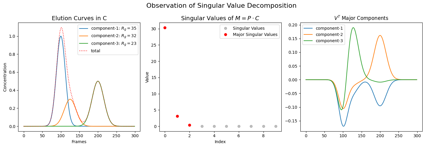
Note that the components on the left do not correspond one-to-one to those on the right, and the proportions of the singular values in the center bear no resemblance to those of the real components.