6.5. Linearly Worsened Errors

from molass import get_version
assert get_version() >= '0.5.0', "This tutorial requires molass version 0.5.0 or higher."
import numpy as np
import matplotlib.pyplot as plt
from molass.SAXS.Models.Formfactors import homogeneous_sphere

q = np.linspace(0.005, 0.3, 100)
Rg = 35
R = np.sqrt(5/3)*Rg

I = homogeneous_sphere(q, R)
fig, ax = plt.subplots()
ax.set_yscale('log')
ax.plot(q, I, label='homogeneous sphere')

[<matplotlib.lines.Line2D at 0x159a611e4e0>]

from molass.SAXS.Theory.DjKinning1984 import S0
I1 = homogeneous_sphere(q, R)
I2 = I1 * S0(q, R)

fig, ax = plt.subplots()
ax.set_yscale('log')
ax.plot(q, I1, label='homogeneous sphere')
ax.plot(q, I2, label='with structure factor S(q)')
ax.legend()

<matplotlib.legend.Legend at 0x159a84f4d40>

import numpy as np
import matplotlib.pyplot as plt
from bisect import bisect_right
from molass.SEC.Models.Simple import gaussian
from molass.LowRank.LowRankInfo import get_denoised_data

def plot_structure_factor(Rg=35, ratio=1.0, error_level=0.05):
    x = np.arange(300)
    q = np.linspace(0.005, 0.3, 200)

    R = np.sqrt(5/3)*Rg
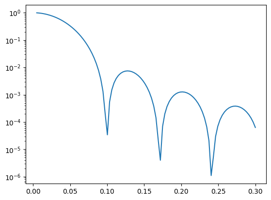
    I1 = homogeneous_sphere(q, R)**2 
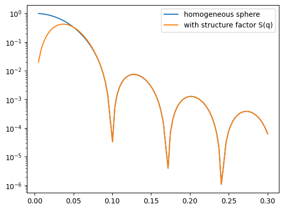
    I2 = I1 * S0(q, R)

    i = bisect_right(q, 0.02)
    h, m, s = 1, 150, 30
    y = gaussian(x, h, m, s)
    fig = plt.figure(figsize=(15,8))
    ax1 = fig.add_subplot(231)
    ax2 = fig.add_subplot(232)
    ax3 = fig.add_subplot(233, projection='3d')
    ax4 = fig.add_subplot(234)
    ax5 = fig.add_subplot(235)
    ax6 = fig.add_subplot(236, projection='3d')

    ax2.set_yscale('log')
    for ax in [ax1, ax2]:
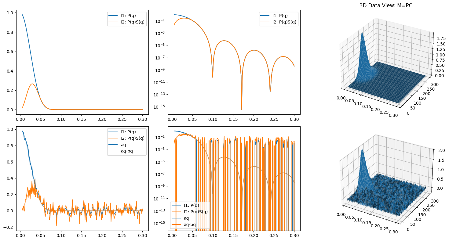
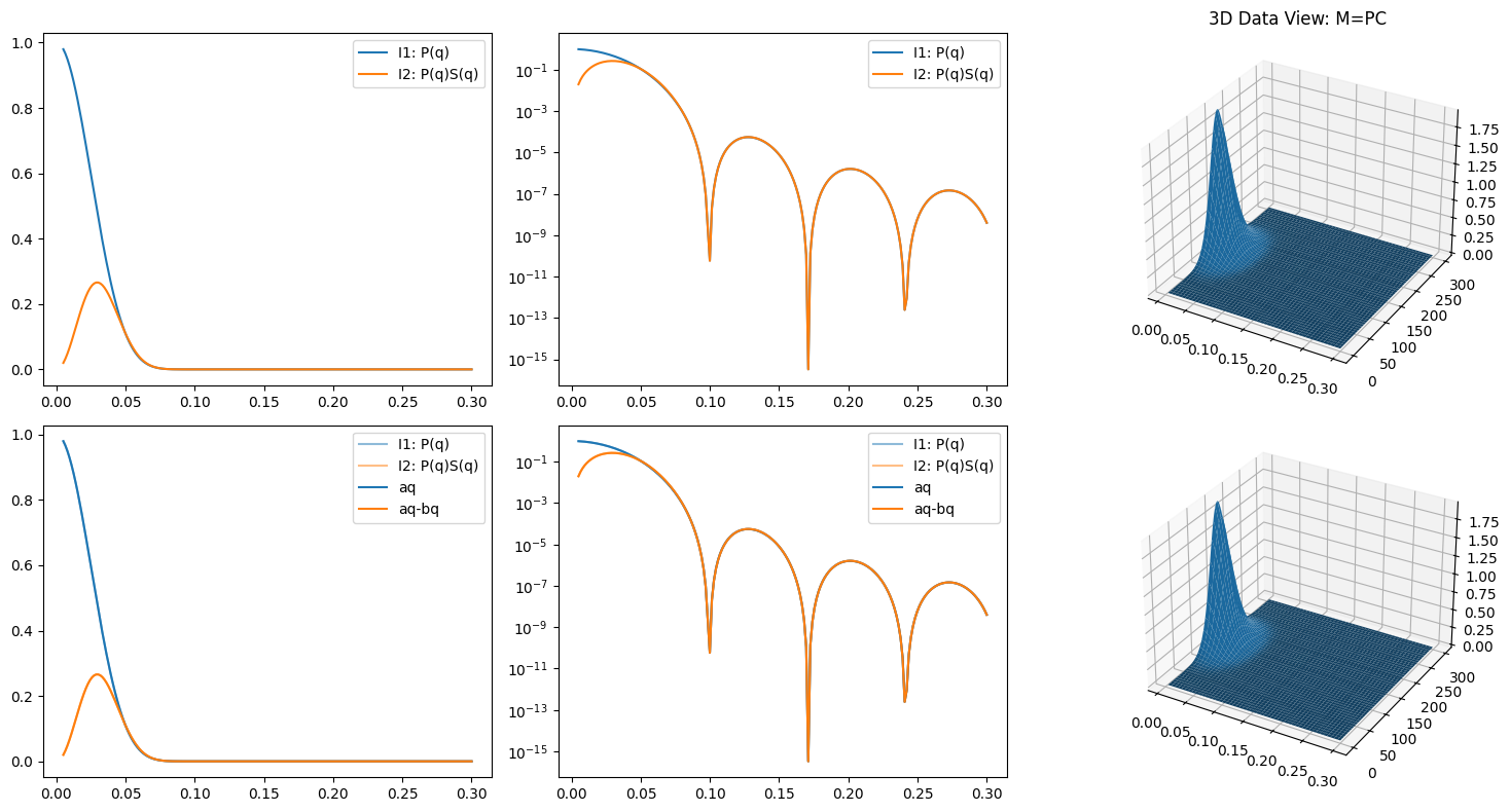
        ax.plot(q, I1, label='I1: P(q)')
        ax.plot(q, I2, label='I2: P(q)S(q)')
        bq = (I1 - I2)*ratio
        # ax.plot(q, bq, label='(I1 - I2)')
        ax.legend()

    P = np.array([I1, bq]).T
    C = np.array([y, y**2])
    M = P @ C                   # matrix multiplication

    Me = M + error_level * np.random.randn(*M.shape)
    # Me_ = get_denoised_data(Me, rank=2)

    # y_ = Me_[i,:]
    # Cinv = np.linalg.pinv(np.array([y_, y_**2]))
    Cinv = np.linalg.pinv(C)
    P_ = Me @ Cinv

    xx, qq = np.meshgrid(x, q)
    ax3.set_title("3D Data View: M=PC")
    ax3.plot_surface(qq, xx, M)
    ax6.plot_surface(qq, xx, Me)
    ax5.set_yscale('log')

    for ax in [ax4, ax5]:
        ax.plot(q, I1, alpha=0.5, label='I1: P(q)')
        ax.plot(q, I2, alpha=0.5, label='I2: P(q)S(q)')
        # ax.plot(q, bq, alpha=0.5, label='(I1 - I2)')
        aq = P_[:,0]
        bq = P_[:,1]
        ax.plot(q, aq, color='C0', label='aq')
        # ax.plot(q, bq, color='C2', label='bq')
        ax.plot(q, aq - bq, color='C1', label='aq-bq')
        ax.legend()
    fig.tight_layout()

plot_structure_factor(error_level=0.05)

plot_structure_factor(error_level=0.0)