Relation between LRF and SVD

Goal and Terminology¶

We have already made the following observations about SVD.

Especially, the second observation strongly indicates that SVD is quite different from the chromatographic decomposition.

In this section, we will confirm or observe the following points.

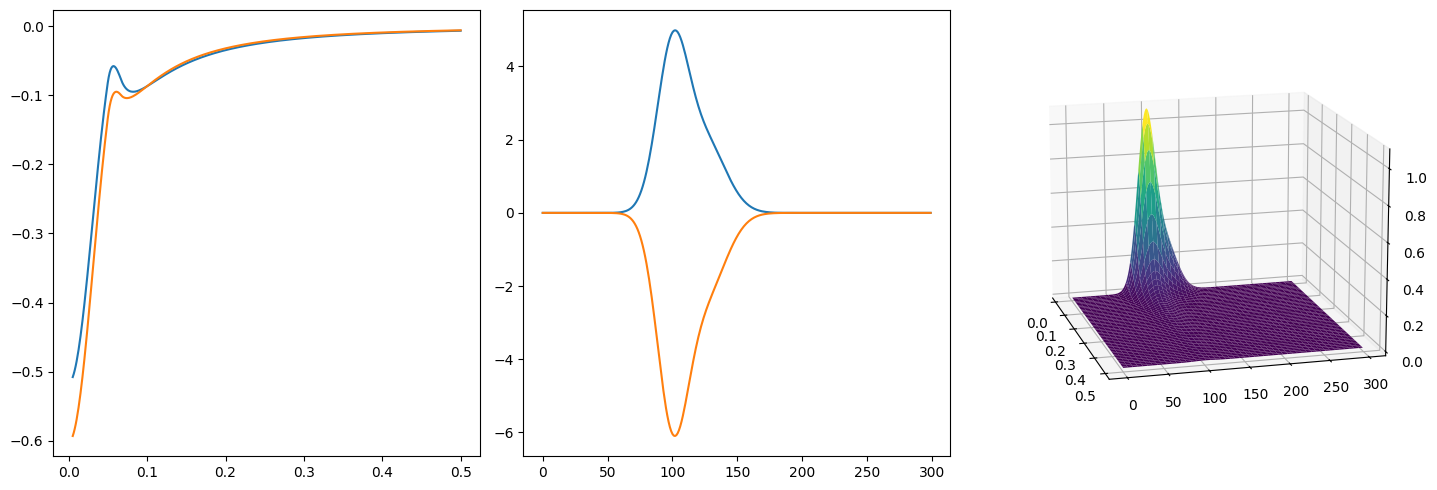
A truncated SVD can be easily (or trivially) transformed to an (unrealistic) example of LRF.
We can generate an infinite number of candedate LRFs from a A truncated SVD.
Every member of the candedate set is equally likely with respect to the matrix norm $\| M - P \cdot C \|$ .
Thus, a chromatogrpahic decomposition, which is the LRF we want, cannot be obtained without some proper constraints.

By “truncated SVD”, we mean here the approximation $M \approx [u_1, u_2, ... u_k] \cdot diag([\sigma_1, \sigma_2, ..., \sigma_k]) \cdot [v_1, v_2, ..., v_k]^T$ , which we will denote just $U \cdot \Sigma \cdot V^T$ .

Dataset for Observation¶

For simplicity, let $k = 2$ and consider the following truncdated SVD.

import numpy as np
import matplotlib.pyplot as plt
from molass.SAXS.Models.Simple import guinier_porod
from molass.SEC.Models.Simple import gaussian

x = np.arange(300)
q = np.linspace(0.005, 0.5, 400)

def plot_multiple_component_data(scattering_params, elution_params, use_matrices=False, view=None, noise=None):
    fig = plt.figure(figsize=(15,5))
    ax1 = fig.add_subplot(131)
    ax2 = fig.add_subplot(132)
    ax3 = fig.add_subplot(133, projection='3d')
    
    fig.suptitle(r"Illustration of Decomposition $M = P \cdot C$ simulated with Guinier-Prod and EGH Models in Molass Library", fontsize=16)

    # ax1.set_yscale('log')
    ax1.set_title("Scattering Curves in P", fontsize=14)
    ax1.set_xlabel("Q")
    ax1.set_ylabel("Intensity")
    w_list = []
    rgs = []
    for i, (G, Rg, d) in enumerate(scattering_params):
        w, q1 = guinier_porod(q, G, Rg, d, return_also_q1=True)
        w_list.append(w)
        color = "C%d" % i
        ax1.plot(q, w, color=color, label='component-%d: $R_g=%.3g$' % (i+1, Rg))
        rgs.append(Rg)
        # ax1.axvline(q1, linestyle=':', color=color, label='Guinier-Porod $Q_1$')
    ax1.legend()

    y_list = []
    ax2.set_title("Elution Curves in C", fontsize=14)
    ax2.set_xlabel("Frames")
    ax2.set_ylabel("Concentration")
    for i, (h, m, s) in enumerate(elution_params):
        y = gaussian(x, h, m, s)
        y_list.append(y)
        ax2.plot(x, y, label='component-%d: $R_g=%.3g$' % (i+1, rgs[i]))
    ty = np.sum(y_list, axis=0)
    ax2.plot(x, ty, ':', color='red', label='total')
    ax2.legend()

    ax3.set_title(r"$M$ calculated by $P \cdot C$", fontsize=14)
    ax3.set_xlabel("Q")
    ax3.set_ylabel("Frames")
    ax3.set_zlabel("Intensity")
    xx, qq = np.meshgrid(x, q)
    if use_matrices:
        P = np.array(w_list).T
        C = np.array(y_list)
        M = P @ C
    else:
        zz_list = []
        for w, y in zip(w_list, y_list):
            zz =  w.reshape((len(q),1)) @ y.reshape((1,len(x)))
            zz_list.append(zz)
        M = np.sum(zz_list, axis=0)
    if noise is not None:
        M += noise * np.random.randn(*M.shape)
    ax3.plot_surface(qq, xx, M, color='red', alpha=0.5)
    # ax3.legend()
    if view is not None:
        ax3.view_init(azim=view[0], elev=view[1])
    Cinv = np.linalg.pinv(C)
    P_ = M @ Cinv
    for py in P_.T:
        ax1.plot(q, py, linestyle=':', color="red")
    fig.tight_layout()
    fig.subplots_adjust(right=0.95)

    return M

rgs = (35, 32)
scattering_params = [(1, rgs[0], 2), (1, rgs[1], 3)]
elution_params = [(1, 100, 12), (0.3, 125, 16)]
M = plot_multiple_component_data(scattering_params, elution_params, use_matrices=True, view=(-15, 15))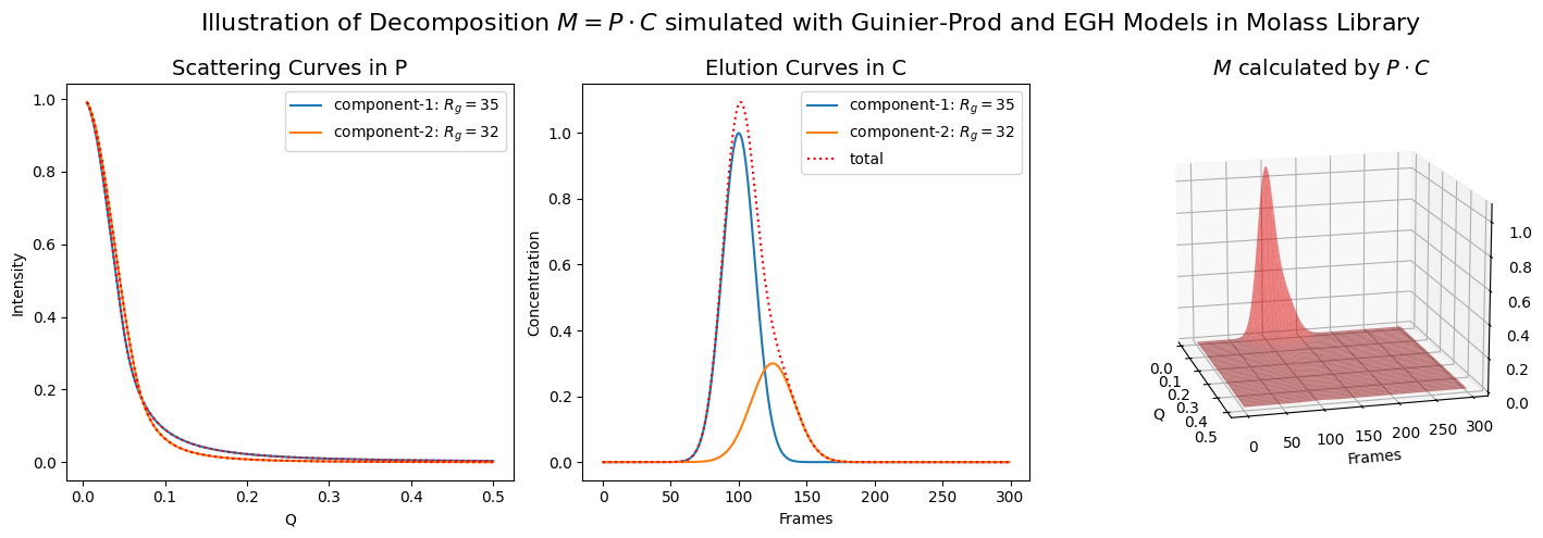

Random LRF Generation¶

k = 2
U, s, VT = np.linalg.svd(M)
U_ = U[:,:k]
s_ = s[:k]
VT_ = VT[:k,:]
M_ = U_ @ np.diag(s_) @ VT_
scales = np.sqrt(s_)
print(M.shape, M_.shape, np.linalg.norm(M - M_), s_, scales)

(400, 300) (400, 300) 1.569660885325227e-14 [26.15172839  0.41368576] [5.11387606 0.64318408]

def plot_any_lrf(A, positive=False, view=None):
    A_ = np.diag(scales) @ A
    P = U_ @ A_
    if positive:
        pass
    Ainv = np.linalg.inv(A)
    Ainv_ = Ainv @ np.diag(scales)
    C = Ainv_ @ VT_
    D = P @ C

    print(A, A @ Ainv)
    print(A_ @ Ainv_, s_)
    print(np.linalg.norm(D - M_))

    fig = plt.figure(figsize=(15,5))
    ax1 = fig.add_subplot(131)
    ax2 = fig.add_subplot(132)
    ax3 = fig.add_subplot(133, projection='3d')

    for py in P.T:
        ax1.plot(q, py)

    for cy in C:
        ax2.plot(x, cy)

    xx, qq = np.meshgrid(x, q)
    ax3.plot_surface(qq, xx, D, cmap='viridis')

    if view is not None:
        ax3.view_init(azim=view[0], elev=view[1])

    fig.tight_layout()
    fig.subplots_adjust(right=0.95)
    plt.show()

plot_any_lrf(np.random.uniform(size=(2,2)), view=(-15, 15))

[[0.41691119 0.50674548]
 [0.92488475 0.76617207]] [[ 1.00000000e+00 -5.70644784e-17]
 [ 1.21024632e-16  1.00000000e+00]]
[[ 2.61517284e+01  6.99175891e-16]
 [-4.28609098e-16  4.13685757e-01]] [26.15172839  0.41368576]
1.0203681502926361e-14

Goal and Terminology¶

Dataset for Observation¶

Random LRF Generation¶

Positive LRF Generation¶