Noise Reduction with SVD - Molass Library Essence

How to Denoise¶

As commonly known Schanze, 2018, we can denoise $M$ by ignoring the insignificant tail^[1] of the following expansion made from SVD - Singular Value Decomposition - based on the linear nature expected in the data.

M = \sum_{i=1}^{n} \sigma_i u_i v_i^* \qquad \qquad (4)

(1)

where

$n \leq \min(rows, columns)$ : the rank of $M$ ,
$\sigma_i$ : ith singular value,
$u_i$ : ith row vector of the unitary matrix usually denoted by $U$ ,
$v_i^*$ : traspose of ith row vector of the unitary matrix usually denoted by $V$ .

Denoise Example¶

To confirm the performance of the denoise method above, let us compare the noisy data and their denoised version.

Our observation strategy is as follows.

Consider a single component case for simplicity
Assume that a true elution curve $C$ is known.
Denoise $M_{noisy}$ into $M_{denoised}$ usign the SVD expansion above
Compute spectral curves $P_{noisy}$ and $P_{denoised}$ from $M_{noisy}$ and $M_{denoised}$ using the inverse of $C$
Compare the computed spectral curves $P_{noisy}$ and $P_{denoised}$

import numpy as np
import matplotlib.pyplot as plt
from molass.SAXS.Models.Simple import guinier_porod
from molass.SEC.Models.Simple import gaussian
from molass.LowRank.LowRankInfo import get_denoised_data

x = np.arange(300)
q = np.linspace(0.005, 0.5, 400)

def plot_single_component_data(scatter_params, elution_params, noise=None):
    G, Rg, d = scatter_params
    h, m, s = elution_params
    fig = plt.figure(figsize=(15,8))
    ax1 = fig.add_subplot(231)
    ax2 = fig.add_subplot(232)
    ax3 = fig.add_subplot(233, projection='3d')
    ax4 = fig.add_subplot(234)
    ax5 = fig.add_subplot(235)
    ax6 = fig.add_subplot(236, projection='3d')

    I, q1 = guinier_porod(q, G, Rg, d, return_also_q1=True)
    # ax1.set_yscale('log')
    for ax in [ax1, ax4]:
        ax.set_title(f"Scattering Curve")
        ax.plot(q, I, label='True $P$')
        ax.axvline(q1, linestyle=':', color="green", label='Guinier-Porod $Q_1$')

    y = gaussian(x, h, m, s)
    for ax in [ax2, ax5]:
        ax.set_title("Elution Curve")
        ax.plot(x, y, label='True $C$')
        ax.legend()

    P = I.reshape((len(q),1))   # make it a matrix
    C = y.reshape((1,len(x)))   # make it a matrix
    M = P @ C                   # matrix multiplication
    if noise is not None:
        M += noise * np.random.randn(*M.shape)
    xx, qq = np.meshgrid(x, q)
    ax3.set_title("3D View: $M_{noisy}$")
    ax3.plot_surface(qq, xx, M)

    Cinv = np.linalg.pinv(C)
    P_ = M @ Cinv
    ax1.plot(q, P_, linestyle=':', color="red", label='$P_{noisy}$')

    D = get_denoised_data(M, rank=1)
    ax6.set_title("3D View: $M_{denoised}$")
    ax6.plot_surface(qq, xx, D)

    Pd = D @ Cinv
    ax4.plot(q, Pd, linestyle=':', color="red", label='$P_{denoised}$')

    for ax in [ax1, ax4]:
        ax.legend()

    fig.tight_layout()

plot_single_component_data((1, 35, 3), (1, 150, 30), noise=0.1)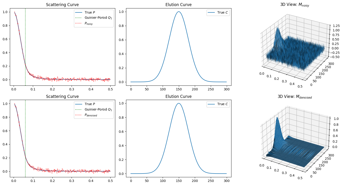

We can observe significant improvement in the 3D views on the right, while the estimated scattering curves on the left look almost the same. The explanation for this gap remains to be resolved. It may indicate a limitation of SVD-based denoising when it comes to improving the estimation of the scattering curve.

Footnotes¶

terms where $n \geq i \geq r$ assuming the target rank is r, which is supposed to be the number of components in cases of simple assumption. Otherwize, e.g, if any significant interparticle effects are suspected, this number should be duly incremented. Molass Library can deal with this issue by adding extra quadratic rows to $C$ when the concentration dependence can be assumed linear.
↩

References¶

Schanze, T. (2018). Compression and Noise Reduction of Biomedical Signals by Singular Value Decomposition. IFAC-PapersOnLine, 51(2), 361–366. https://doi.org/10.1016/j.ifacol.2018.03.062