Proportional EGH Modeling - Molass Library Essence

How to Modify the Component Proportions¶

First, let us introduce what we think are the standard steps as follows.

Default decomposition
Show the default proportions
Decompose with modified proportions
Confirm by comparison Plot

from molass import get_version
assert get_version() >= '0.7.0', "This tutorial requires molass version 0.7.0 or higher."
from molass_data import SAMPLE1
from molass.DataObjects import SecSaxsData as SSD
ssd = SSD(SAMPLE1)
trimmed_ssd = ssd.trimmed_copy()
corrected_ssd = trimmed_ssd.corrected_copy()
decomposition = corrected_ssd.quick_decomposition(num_components=3)
decomposition.plot_components(title="Default Decomposition into 3 Components");

zeros at the angular ends of error data have been replaced with the adjacent values.

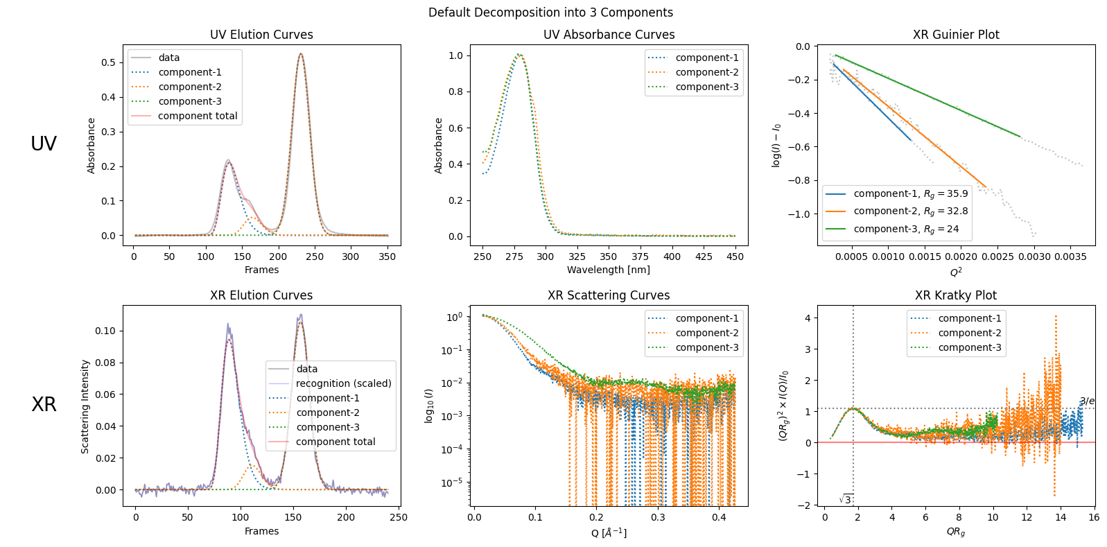
proportions = decomposition.get_proportions()
proportions

array([0.44395829, 0.07063981, 0.4854019 ])

modified_decomposition = corrected_ssd.quick_decomposition(num_components=3, proportions=[0.32, 0.20, 0.48])

from molass.PlotUtils.Comparison import comparison_plot
comparison_plot([decomposition, modified_decomposition], title="Comparison of Decompositions", show_proportions=True)

Proportions of the first decomposition: [0.44395829 0.07063981 0.4854019 ]
Proportions of the second decomposition: [0.31999337 0.19999916 0.48000747]

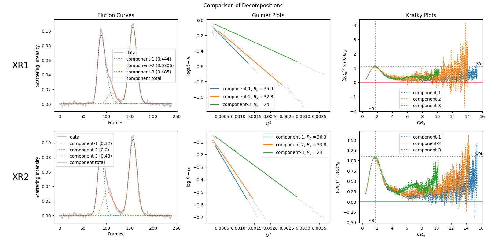
In this comparison plot, we can compare the propotions easily.

How to Vary the Component Proportions¶

In the previous example, we could be reasonably confident about the number of components, to a certain extent, based on the observation of the elution curve. However, that is not always the case. To illustrate this, let us consider another example where we cannot be so confident.

Below, we will decompose another sample in two ways: first into two components, and then into three components. We will also vary the proportions using another utility function.

Preparation¶

For effective observation, we will also prepare the Rg curve.

from molass_data import SAMPLE4
from molass.DataObjects import SecSaxsData as SSD
ssd = SSD(SAMPLE4)
trimmed_ssd = ssd.trimmed_copy()
corrected_ssd = trimmed_ssd.corrected_copy()
rgcurve = corrected_ssd.xr.compute_rgcurve()

Varying Proportions into Two Components¶

import numpy as np
num_trails = 8
species1_proportions = np.ones(num_trails) * 3
species2_proportions = np.linspace(1, 3, num_trails)
proportions = np.array([species1_proportions, species2_proportions]).T
proportions

array([[3.        , 1.        ],
       [3.        , 1.28571429],
       [3.        , 1.57142857],
       [3.        , 1.85714286],
       [3.        , 2.14285714],
       [3.        , 2.42857143],
       [3.        , 2.71428571],
       [3.        , 3.        ]])

corrected_ssd.plot_varied_decompositions(proportions, rgcurve=rgcurve, best=3);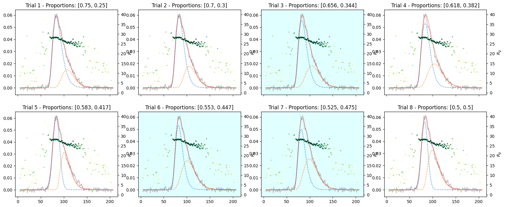

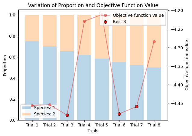
Varying Proportions into Three Components¶

species3_proportions = np.ones(num_trails) * 1
proportions = np.array([species1_proportions, species2_proportions, species3_proportions]).T
proportions

array([[3.        , 1.        , 1.        ],
       [3.        , 1.28571429, 1.        ],
       [3.        , 1.57142857, 1.        ],
       [3.        , 1.85714286, 1.        ],
       [3.        , 2.14285714, 1.        ],
       [3.        , 2.42857143, 1.        ],
       [3.        , 2.71428571, 1.        ],
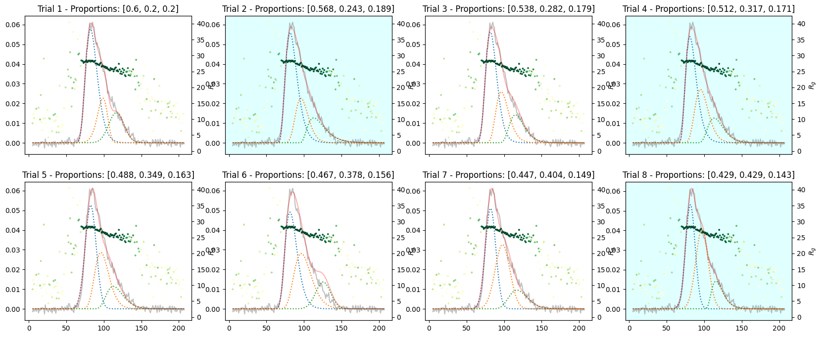
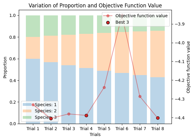
       [3.        , 3.        , 1.        ]])

corrected_ssd.plot_varied_decompositions(proportions, rgcurve=rgcurve, best=3);