Sphere Scattering - Molass Library Essence

Following Pedersen, 1997, we will glance over the model.

F_1(q,R) = \frac{3[\sin(q R) - q R \cos(q R)]}{(q R)^3}

(1)

from molass import get_version
assert get_version() >= '0.6.0', 'Please update molass to the latest version'
import numpy as np
import matplotlib.pyplot as plt
from molass.SAXS.Models.Formfactors import homogeneous_sphere

q = np.linspace(0.005, 0.7, 100)
R = 30

I = homogeneous_sphere(q, R)**2
fig, (ax1, ax2) = plt.subplots(ncols=2, figsize=(10, 5))
ax2.set_yscale('log')
for ax in ax1, ax2:
    ax.plot(q, I, label='homogeneous sphere')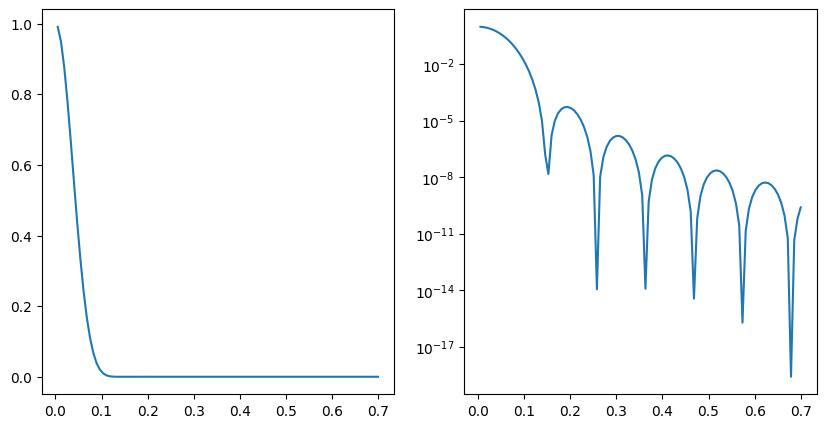

References¶

Pedersen, J. S. (1997). Analysis of small-angle scattering data from colloids and polymer solutions: modeling and least-squares fitting. Advances in Colloid and Interface Science, 70, 171–210. https://doi.org/10.1016/S0001-8686(97)00312-6