9. Nontrivial Decomposition

This chapter will discuss the cases where component peaks are not apparent.

9.1. Initial Observation

Let us first observe such an example.

from molass import get_version
assert get_version() >= '0.6.0', "This tutorial requires molass version 0.6.0 or higher."
from molass_data import get_version
assert get_version() >= '0.3.0', "This tutorial requires molass_data version 0.3.0 or higher."
from molass_data import SAMPLE4
from molass.DataObjects import SecSaxsData as SSD
ssd = SSD(SAMPLE4)
trimmed_ssd = ssd.trimmed_copy()
corrected_ssd = trimmed_ssd.corrected_copy()
corrected_ssd.plot_compact();

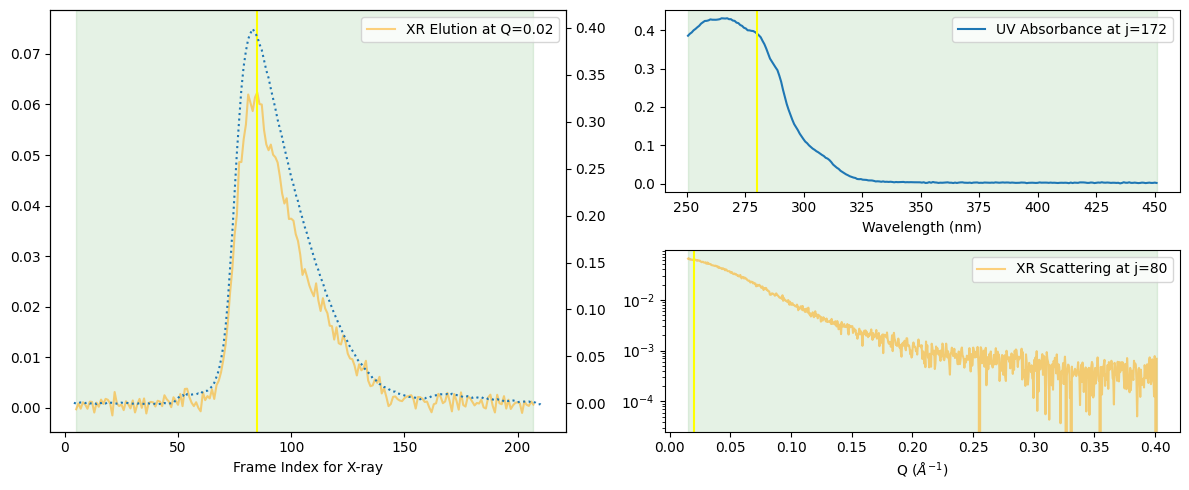
At first glance, the peak may seem to consist of a single component. For a more detailed observation, let us assume it may consist of two components and add the Rg curve.

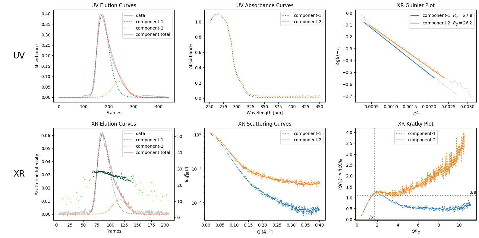
rgcurve = corrected_ssd.xr.compute_rgcurve()
decomposition = corrected_ssd.quick_decomposition(num_components=2)
decomposition.plot_components(rgcurve=rgcurve)

100%|██████████| 203/203 [00:07<00:00, 25.46it/s]

<molass.PlotUtils.PlotResult.PlotResult at 0x24a368a6f60>

9.2. Varied Binary Proportions

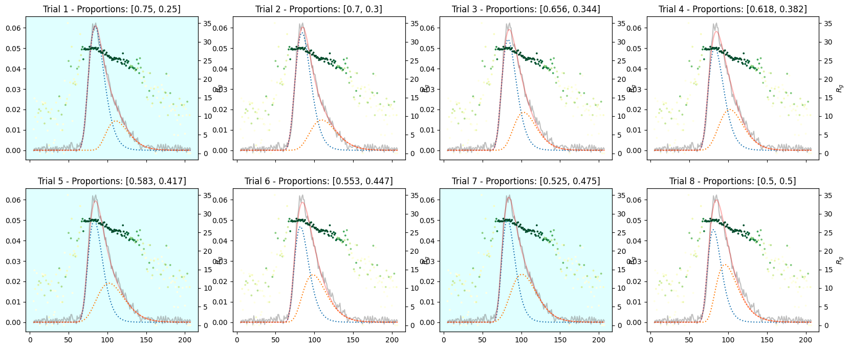
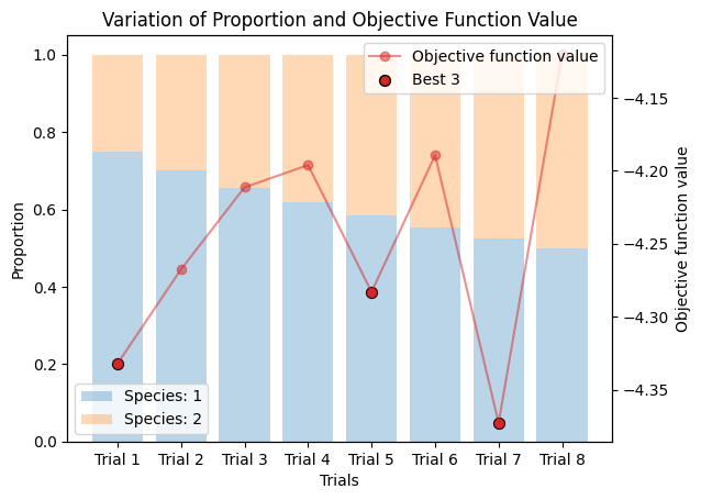
If you are not sure about the default compositiun, you can compare the results with different proportions as follows.

import numpy as np
num_trails = 8
species1_proportions = np.ones(num_trails) * 3
species2_proportions = np.linspace(1, 3, num_trails)
proportions = np.array([species1_proportions, species2_proportions]).T
proportions

array([[3.        , 1.        ],
       [3.        , 1.28571429],
       [3.        , 1.57142857],
       [3.        , 1.85714286],
       [3.        , 2.14285714],
       [3.        , 2.42857143],
       [3.        , 2.71428571],
       [3.        , 3.        ]])

corrected_ssd.plot_varied_decompositions(proportions, rgcurve=rgcurve, best=3)

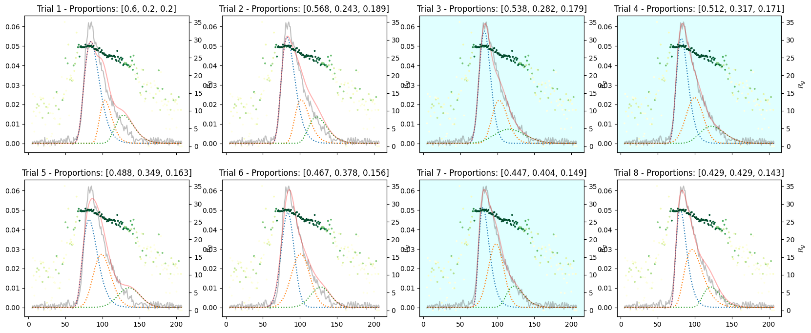
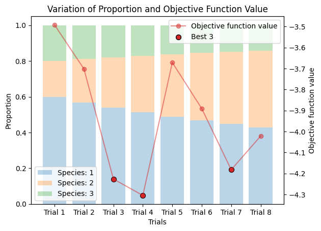
9.3. Varied Tertiary Proportions

If the existence of three components are suspected, do as follows.

species3_proportions = np.ones(num_trails) * 1
proportions = np.array([species1_proportions, species2_proportions, species3_proportions]).T
proportions

array([[3.        , 1.        , 1.        ],
       [3.        , 1.28571429, 1.        ],
       [3.        , 1.57142857, 1.        ],
       [3.        , 1.85714286, 1.        ],
       [3.        , 2.14285714, 1.        ],
       [3.        , 2.42857143, 1.        ],
       [3.        , 2.71428571, 1.        ],
       [3.        , 3.        , 1.        ]])

corrected_ssd.plot_varied_decompositions(proportions, rgcurve=rgcurve, best=3)