7. Electron Density Retrieval#
SAXS Theory explaines how the X-ray beam is scattered by the sample particles. Our final analysis step is to solve the inverse problem of determining the particle shape or its electron density from a scattering curve which has been so far computed to be a good representation of the scattered X-ray intensities.
For this purpose, DENSS is now the most trusted program in the open source software, for which Molass has a simple wrapper as shown below.
7.1. Learning Points#
jcurve_array = decomposition.get_xr_components()[0].get_jcurve_array()
run_denss(jcurve_array)
show_mrc(‘denss_result.mrc’)
7.2. How to Run DENSS#
First, get a better scattering curve by decomposition.
from molass import get_version
assert get_version() >= '0.6.3', "This tutorial requires molass version 0.6.3 or higher."
from molass_data import SAMPLE1
from molass.DataObjects import SecSaxsData as SSD
ssd = SSD(SAMPLE1)
trimmed_ssd = ssd.trimmed_copy()
corrected_ssd = trimmed_ssd.corrected_copy()
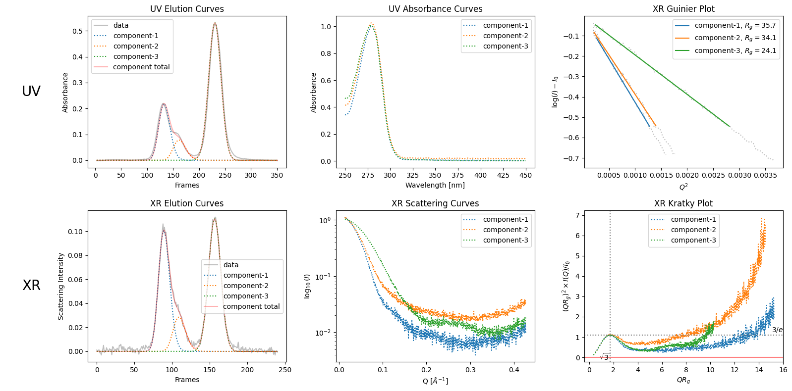
decomposition = corrected_ssd.quick_decomposition(num_components=3)
decomposition.plot_components()
zeros at the angular ends of error data have been replaced with the adjacent values.
<molass.PlotUtils.PlotResult.PlotResult at 0x1c7e1c052b0>
Then, selecting one of the components, run DENSS as follows.
from molass.SAXS.DenssTools import run_denss
# Get, for example, the first component's scattering curve as an array
jcurve_array = decomposition.get_xr_components()[0].get_jcurve_array()
output_folder = "temp"
run_denss(jcurve_array, output_folder=output_folder)
WARNING: Only 2 columns given. Data should have 3 columns: q, I, errors.
WARNING: Setting error bars to 1.0 (i.e., ignoring error bars)


 Step     Chi2     Rg    Support Volume
 ----- --------- ------- --------------
  620   2.94e-02 64.84        1038353
switched to shrinkwrap by density threshold = 0.2000
  999   1.91e-04 35.66        350603          EC: 1 -> 1
 9999   1.49e-05 36.16        313038
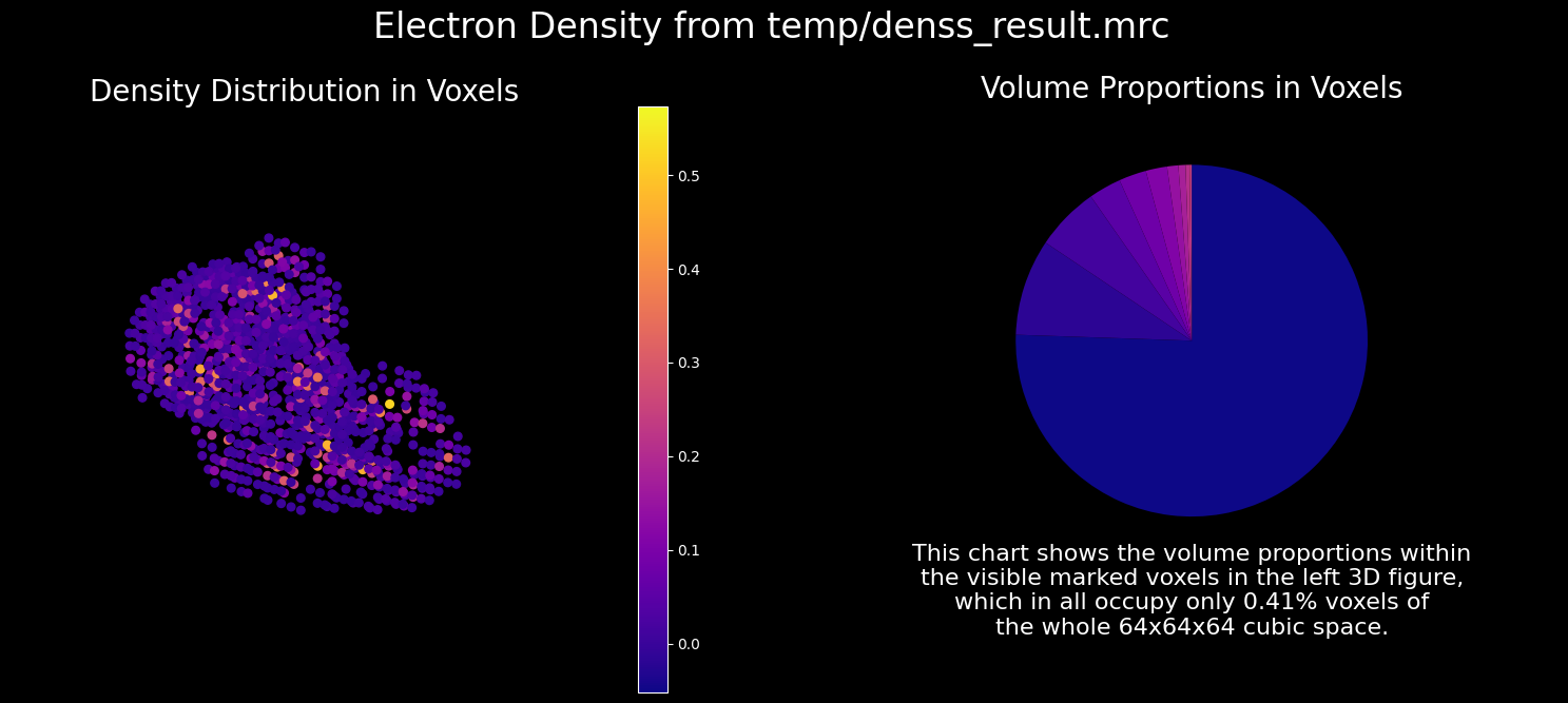
7.3. How to Show the Result#
The result can be visualized as follows.
import matplotlib.pyplot as plt
from molass.SAXS.MrcViewer import show_mrc
# %matplotlib widget
%matplotlib inline
show_mrc(output_folder + '/denss_result.mrc');