Central Moment - Molass Library Essence

This section is a numerical introduction to the concept of central moment in the chromatographic context. Symbolic calculation will later be introduced using SymPy.

Simple Numerical Examples¶

By “chromatographic context”, the following points are suggested.

We will consider the averaging of retention time (x axes in the following figures),
weighted by concentration (y axes).

Uniformly weighted Average¶

import numpy as np
import matplotlib.pyplot as plt

N = 5
x = np.arange(N)
w = np.ones(N)     # uniform weights
plt.bar(x, w)
m = np.mean(x)
s = np.std(x)
plt.axvline(m, color='red')
for p in m-s, m+s:
    plt.axvline(p, color='yellow')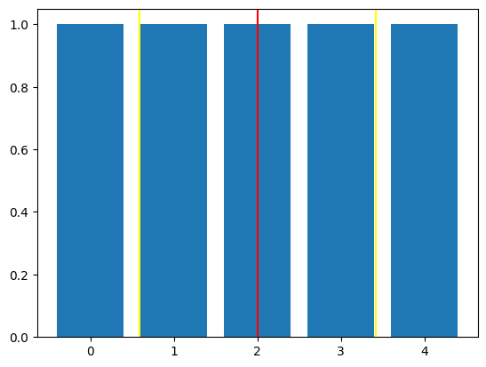

Averaging with Guassian Weights¶

w = np.exp(-(x-2.2)**2)    # non-uniform (gaussian) weights

u = 0
v = 0
for i in range(N):
    u += w[i]*x[i]
    v += w[i]

m = u/v

z = 0
v = 0
for i in range(N):
    z += w[i]*(x[i] - m)**2
    v += w[i]
    
v, z, z/v, np.sqrt(z/v)

s = np.sqrt(z/v)
plt.bar(x, w)
plt.axvline(m, color='red')
for p in m-s, m+s:
    plt.axvline(p, color='yellow')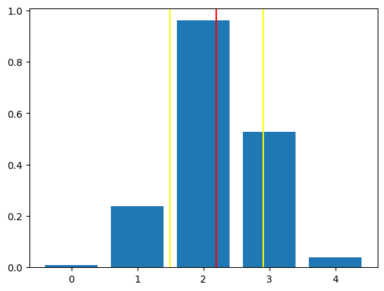

Do it faster in NumPy¶

0th Raw Moment¶

M0 = np.sum(w)
M0

np.float64(1.772080571028074)

1st Raw Moment or Mean¶

M1 = np.sum(w*x)/M0
M1

np.float64(2.199132225263884)

2nd Central Moment and Standard Deviation¶

M2 = np.sum(w*(x - M1)**2)/M0
M2, np.sqrt(M2)

(np.float64(0.49785237938665794), np.float64(0.7055865498906976))