This chapter will discuss the cases where component peaks are not apparent.
Initial Observation
Let us first observe such an example.
from molass import get_version
assert get_version() >= '0.6.0', "This tutorial requires molass version 0.6.0 or higher."
from molass_data import get_version
assert get_version() >= '0.3.0', "This tutorial requires molass_data version 0.3.0 or higher."
from molass_data import SAMPLE4
from molass.DataObjects import SecSaxsData as SSD
ssd = SSD(SAMPLE4)
trimmed_ssd = ssd.trimmed_copy()
corrected_ssd = trimmed_ssd.corrected_copy()
corrected_ssd.plot_compact();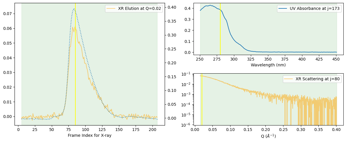
At first glance, the peak may seem to consist of a single component. For a more detailed observation, let us assume it may consist of two components and add the Rg curve.
rgcurve = corrected_ssd.xr.compute_rgcurve()
decomposition = corrected_ssd.quick_decomposition(num_components=2)
decomposition.plot_components(rgcurve=rgcurve)<molass.PlotUtils.PlotResult.PlotResult at 0x25f53c28190>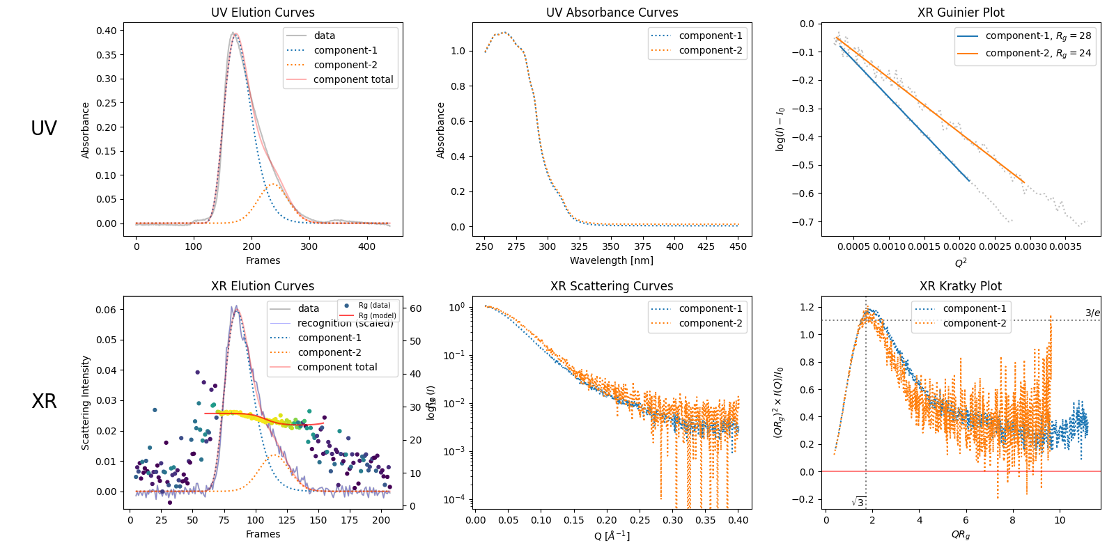
Varied Binary Proportions
When component peaks overlap heavily, the default decomposition may produce inconsistent results depending on noise, because its peak-recognition initialization struggles to distinguish merged peaks.
The proportions option provides a more robust alternative.
It takes a list of approximate area ratios (one per component)
and uses a proportional decomposition algorithm that divides the elution curve
by cumulative area, providing better initialization for the optimizer.
The values do not need to be normalized or exact; for example,
[1, 1], [0.5, 0.5], and [3, 3] all give the same result.
Even a rough estimate like [2, 1] when the true ratio is [1, 1]
is usually sufficient.
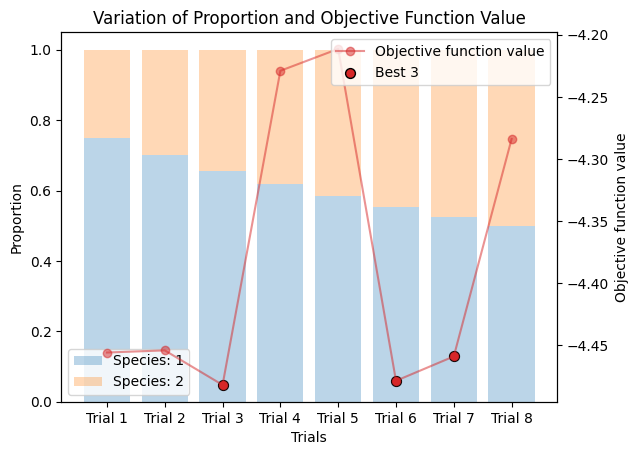
To systematically explore which proportions work best,
you can use plot_varied_decompositions() as follows.
import numpy as np
num_trails = 8
species1_proportions = np.ones(num_trails) * 3
species2_proportions = np.linspace(1, 3, num_trails)
proportions = np.array([species1_proportions, species2_proportions]).T
proportions
array([[3. , 1. ],
[3. , 1.28571429],
[3. , 1.57142857],
[3. , 1.85714286],
[3. , 2.14285714],
[3. , 2.42857143],
[3. , 2.71428571],
[3. , 3. ]])corrected_ssd.plot_varied_decompositions(proportions, rgcurve=rgcurve, best=3)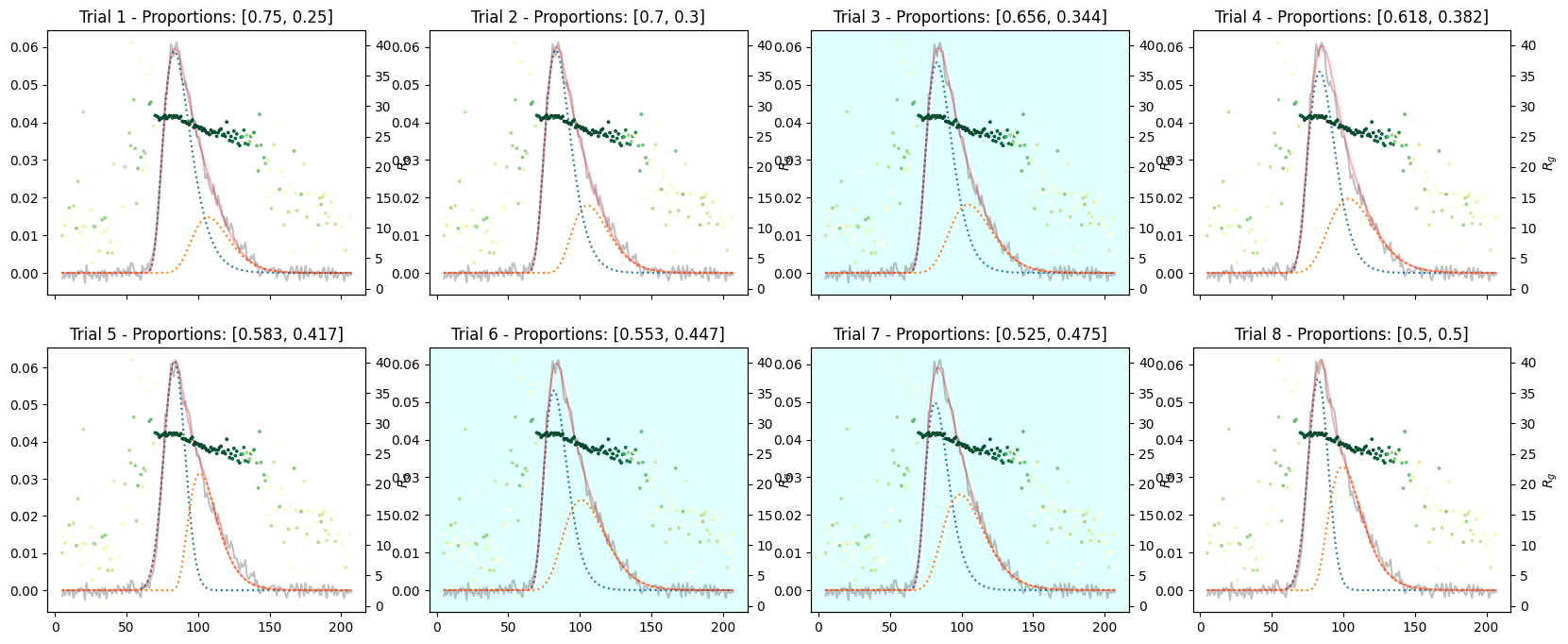
Varied Tertiary Proportions
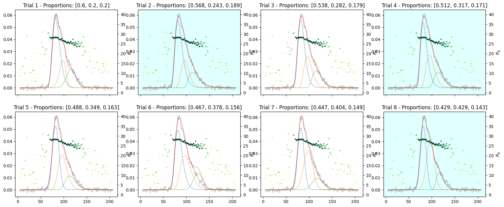
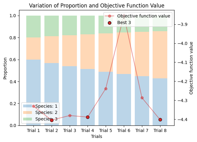
The same approach works for three or more components. If the existence of three components is suspected, extend the proportions array with a third column.
species3_proportions = np.ones(num_trails) * 1
proportions = np.array([species1_proportions, species2_proportions, species3_proportions]).T
proportions
array([[3.        , 1.        , 1.        ],
       [3.        , 1.28571429, 1.        ],
       [3.        , 1.57142857, 1.        ],
       [3.        , 1.85714286, 1.        ],
       [3.        , 2.14285714, 1.        ],
       [3.        , 2.42857143, 1.        ],
       [3.        , 2.71428571, 1.        ],
       [3.        , 3.        , 1.        ]])
corrected_ssd.plot_varied_decompositions(proportions, rgcurve=rgcurve, best=3)