Quick Start: Your First Analysis

This walks through a complete SEC-SAXS decomposition from a cold start, using the sample dataset (SAMPLE1) bundled with the portable download, so you can follow along immediately — no data of your own required yet.

If you haven’t installed Molass GUI, see Installation first.

What you’ll see at the end

A mixture that looks at first glance like two components resolved into three — because one of those two peaks has a smaller shoulder hiding inside it — each with its own separated scattering profile, cross-checked against its own radius of gyration ($R_g$). The same kind of result you’d get from the notebook/API tutorial, but driven entirely by clicking through windows.

0. Launch

Double-click molass-gui.bat. The launcher opens:

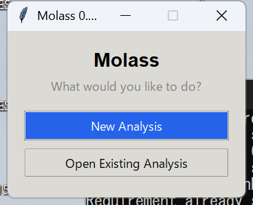
Click New Analysis.

1. Setup: point it at your data

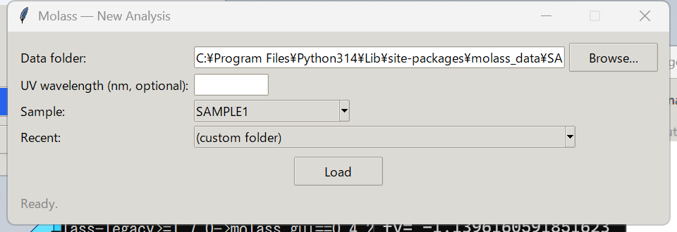
• Data folder: the folder containing your SEC-SAXS measurement files.
• Sample: if the bundled sample data is available (it is, in the portable download), pick SAMPLE1 here instead of typing a path — it fills in the Data folder box for you.
• Leave UV wavelength blank unless you know you need a non-default value.

Click Load.

2. Naive View: how many components?

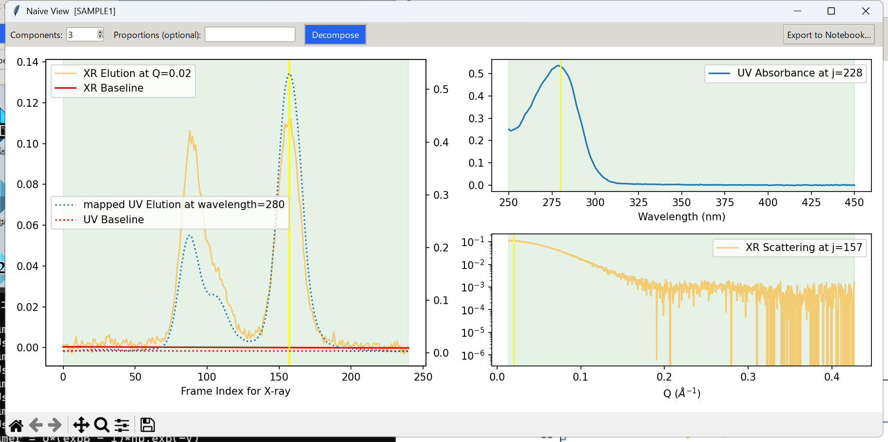
This is the raw data: the X-ray elution curve (orange), the UV-mapped elution curve (blue dots), and each channel’s own profile at the frame marked by the yellow line. Molass already suggests a starting value for Components, computed from the data itself — but look at the plot before accepting it.

For SAMPLE1, two peaks are obviously visible — but look closely at the left-hand peak’s shoulder: there’s a smaller bump riding on it. Fitting it as part of the same component would blur two real, distinct scattering species into one averaged profile, so set Components to 3, not 2. This is the single most important judgment call in the whole workflow — everything downstream builds on it — and it’s a judgment only you, looking at the actual peak shape, can make well. See molass’s own documentation for how to read less obvious cases (overlapping peaks, shoulders, trailing edges).

Click Decompose.

3. Quick Optimization View: review, then upgrade

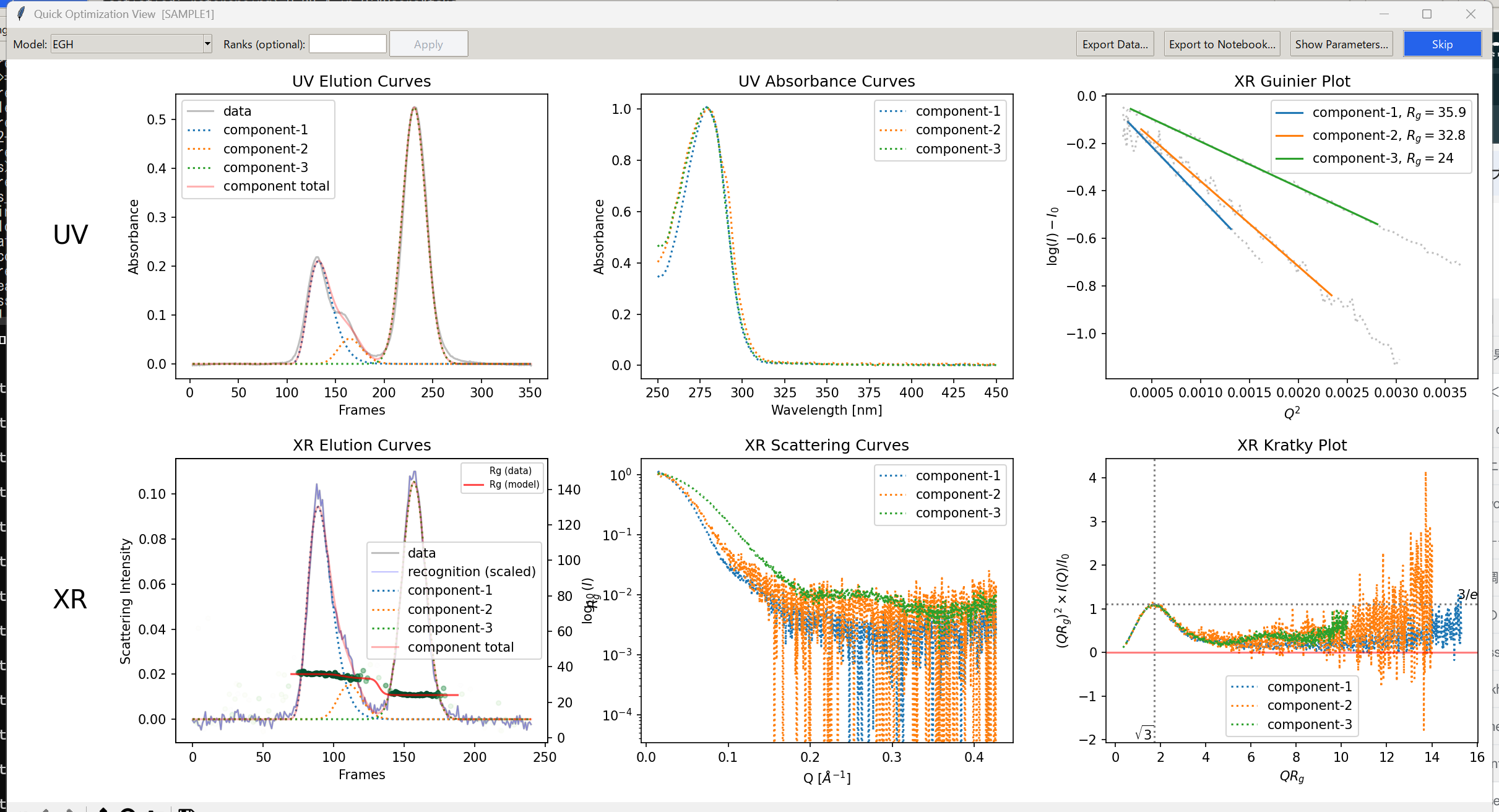
Six panels, all from the same decomposition: elution curves and scattering curves for both UV and X-ray channels, plus a Guinier plot ($R_g$ per component) and a Kratky plot. The default EGH model is purely empirical — a flexible peak shape with no physical column model behind it — fast, and a reasonable sanity check, but not yet using everything Molass can do.

This is also where the small bump becomes its own labeled component (component-2, orange) instead of being folded into its neighbor — confirming that the components-count judgment call above was the right one.

To use one of Molass’s physics-based column models instead (the actual “Upgrade” in Molass’s name), choose one from the Model dropdown — for example EGH → SDM (mono). The button in the top-right corner changes from Skip to Upgrade. Click it.

4. Upgraded View: a physically-constrained fit

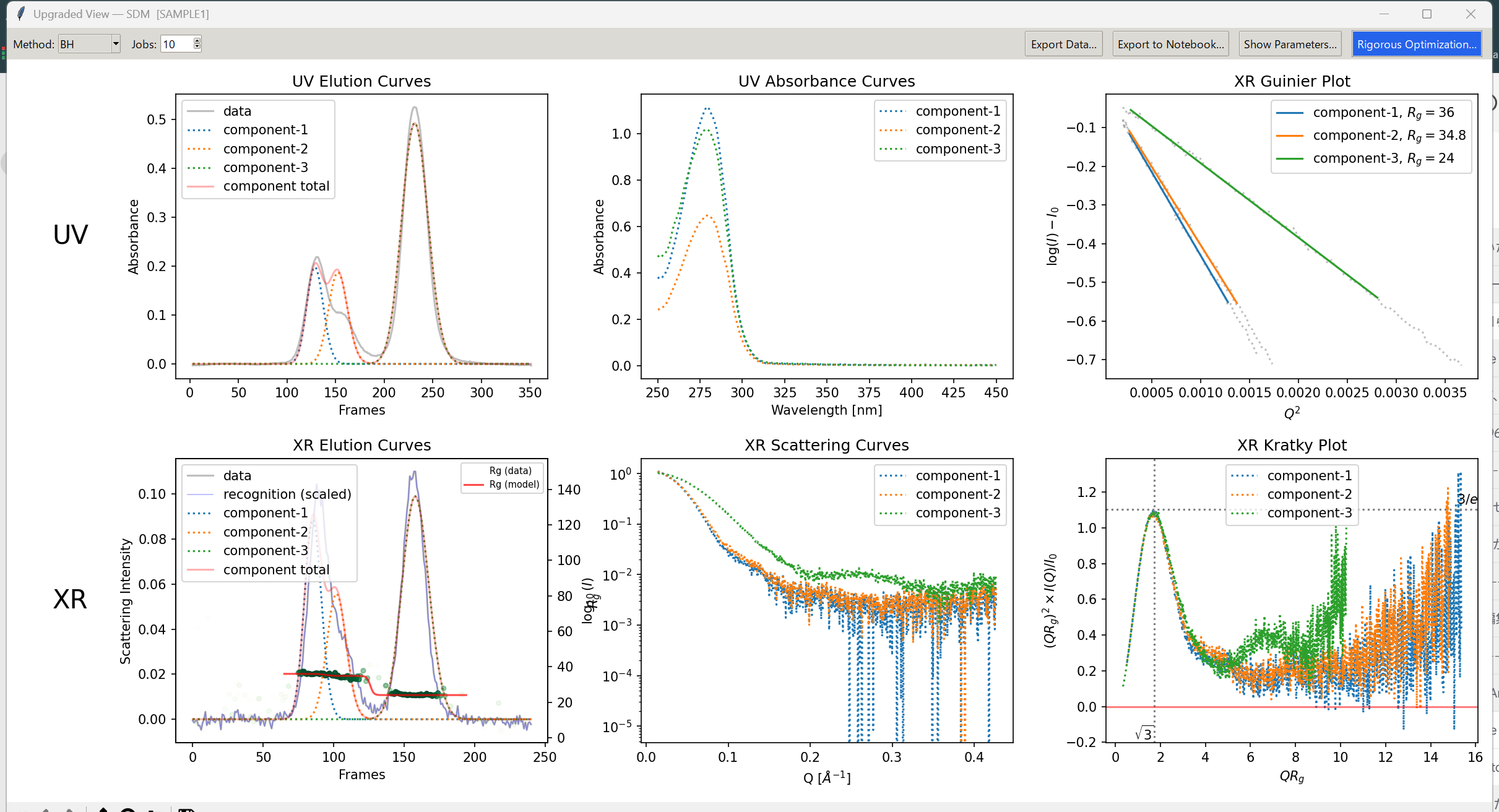
Same six panels, now fit with the column model you chose — in this example, SDM (Stochastic Dispersive Model), which ties each component’s elution shape to actual column-transport physics (pore size, dispersion) rather than an unconstrained empirical curve.

Pick an optimization Method (BH = Basin-Hopping, DE = Differential Evolution — BH is a reasonable default), leave Jobs at its default, and click Rigorous Optimization…. You’ll be asked to choose an output folder for the results — pick anywhere you like.

5. Rigorous Optimization View: watch it refine

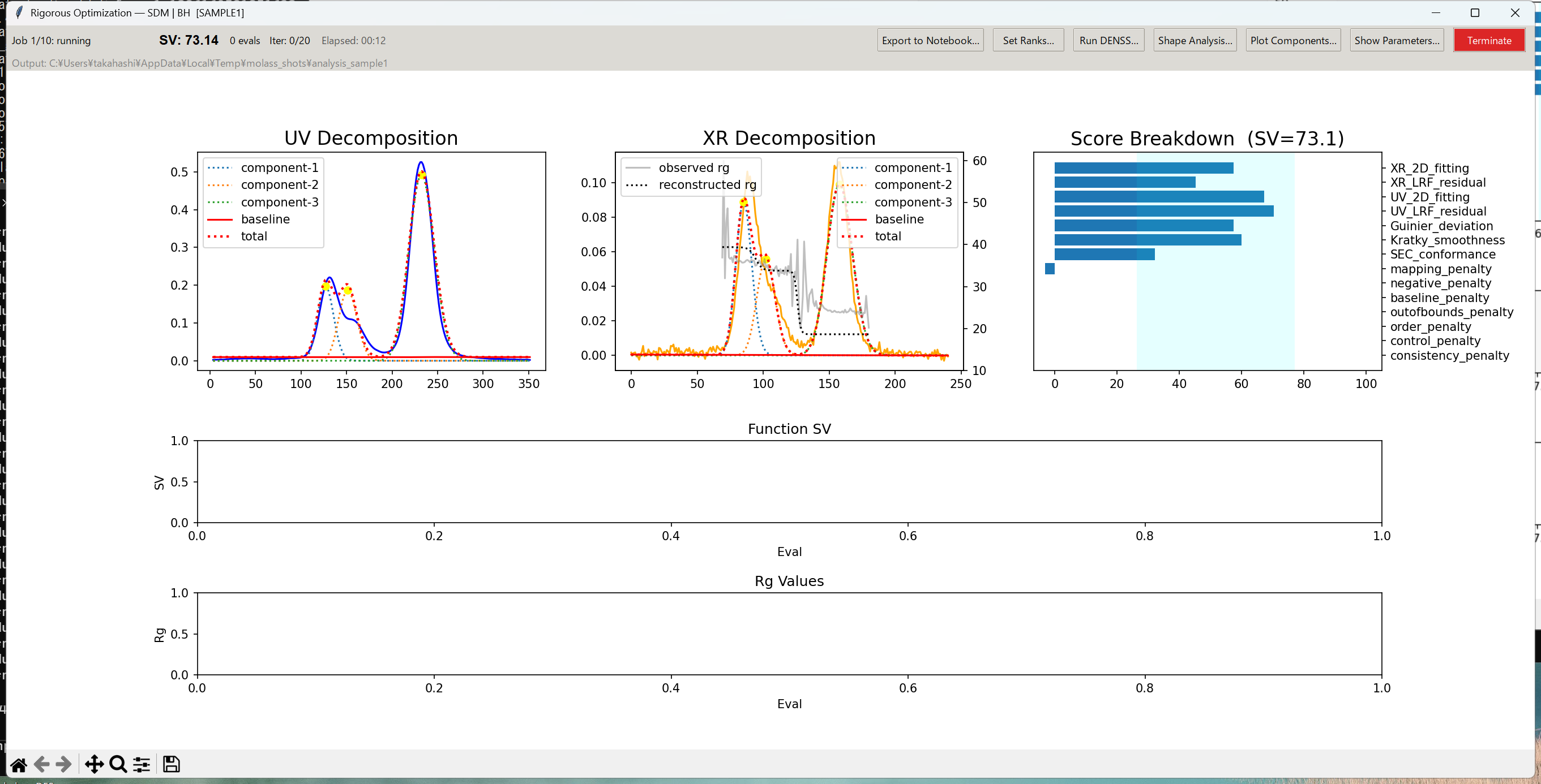
This is a live monitor, not a static report. As soon as the $R_g$ curve finishes computing, an initial score is drawn and optimization starts automatically in the background (you don’t need to click anything else) — the panel shown here is from just a few seconds in. Watch the Score Breakdown bars shrink and the two bottom history plots fill in as iterations proceed; Terminate stops it early if you don’t want to wait for the full run, and Resume restarts a stopped run from where it left off.

When it’s done, use Run DENSS… for 3D shape reconstruction, Shape Analysis… or Plot Components… to inspect the final result, or Export to Notebook… at any phase to continue in a real Jupyter notebook — the escape hatch for anything this wizard doesn’t expose a button for.

Next steps

• Try your own data instead of SAMPLE1 — same five steps.
• Read molass-library’s documentation to understand what each of the five column models (EGH, SDM, EDM, LKM, GRM) actually represents physically.
• If something looks wrong or confusing, please open an issue — reports from people trying this for the first time are exactly what make this guide (and the program) better.